This post is about Exponential Smoothing method, a prediction method for time series data. There are many forms of Exponential Smoothing method and the most basic ones are Single, Double and Triple (Holt-Winters) Exponential Smoothing. Some of the Exponential Smoothing forms can be written as ARIMA model; some of them can not and vice versa. Compared to ARIMA model, Exponential Smoothing method do not have strong model assumptions and it also can not add explanatory variables in the algorithm. However, it is because of its loose model restrictions, Exponential Smoothing can be calculated really fast which is good when you need to predict the value of the next really small period of time like next minute or next five minutes (the time is so short for you to fit a complete ARIMA model). hod.
This post is my note about learning Exponential Smoothing. All the contents in this post are based on my reading on many resources which are listed in the References part.
References
- Paper
- Winters, Peter R. “Forecasting sales by exponentially weighted moving averages.” Management Science 6, no. 3 (1960): 324-342.
- Gardner, E. S. “Smoothing methods for short-term planning and control.” The handbook of forecasting–a manager’s guide (1987): 174-175.
- Taylor, James W. “Short-term electricity demand forecasting using double seasonal exponential smoothing.” Journal of the Operational Research Society 54, no. 8 (2003): 799-805.
- Taylor, James W. “An evaluation of methods for very short-term load forecasting using minute-by-minute British data.” International Journal of Forecasting 24, no. 4 (2008): 645-658.
- Dimitrov, Preslav Encontros Científicos. “Long-run forecasting of the number of the ecotourism arrivals in the municipality of Stambolovo, Bulgaria.” Tourism & Management Studies, (2013), Issue 1, pp.41-47
- Book
- Online Materials
Details
Notations
Define\[ \begin{align} y_t &: \text{the observed data in time }t \\[5pt] \hat{y_t} &: \text{the predicted data in time }t \\[5pt] h &: \text{Number of periods for forecasting} \end{align} \]
Stationary Data
The following graph and explanations can be found in the post, A Complete Tutorial on Time Series Modeling in R which is from the blog, Analytics Vidhya.
- The mean of the series data should be constant and can not be explained by time
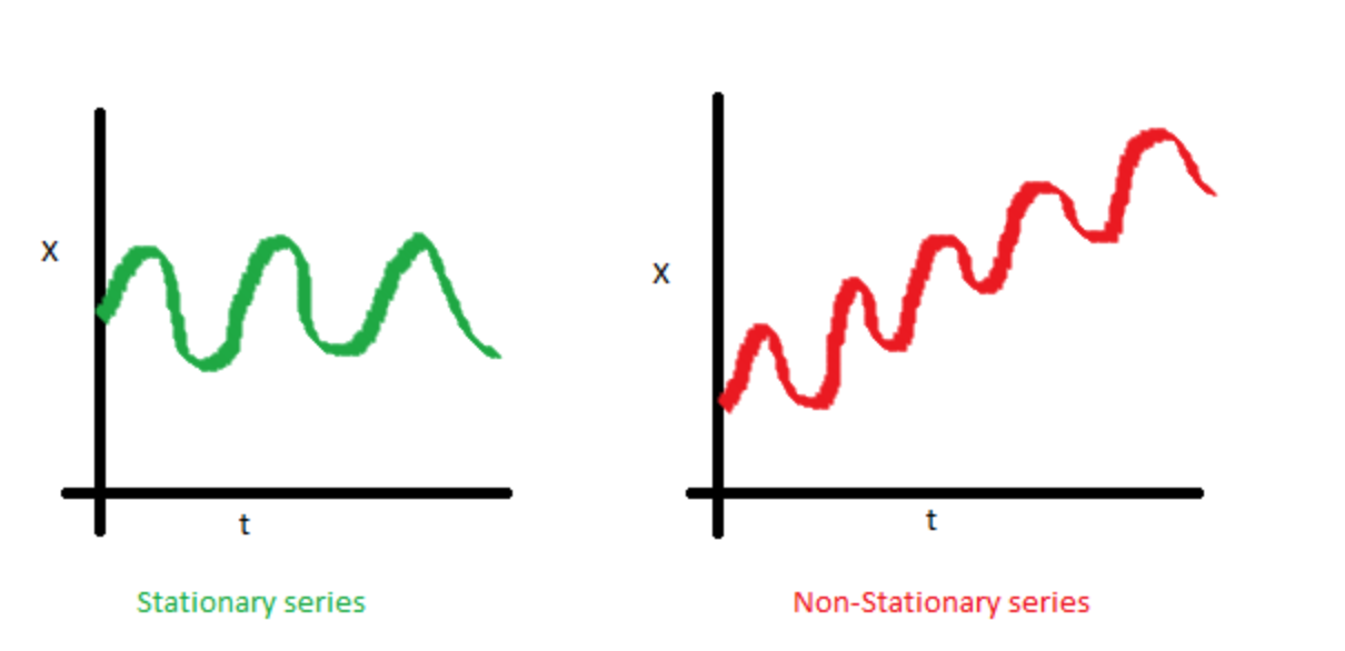
- The variance of the series data should be constant and can not be explained by time
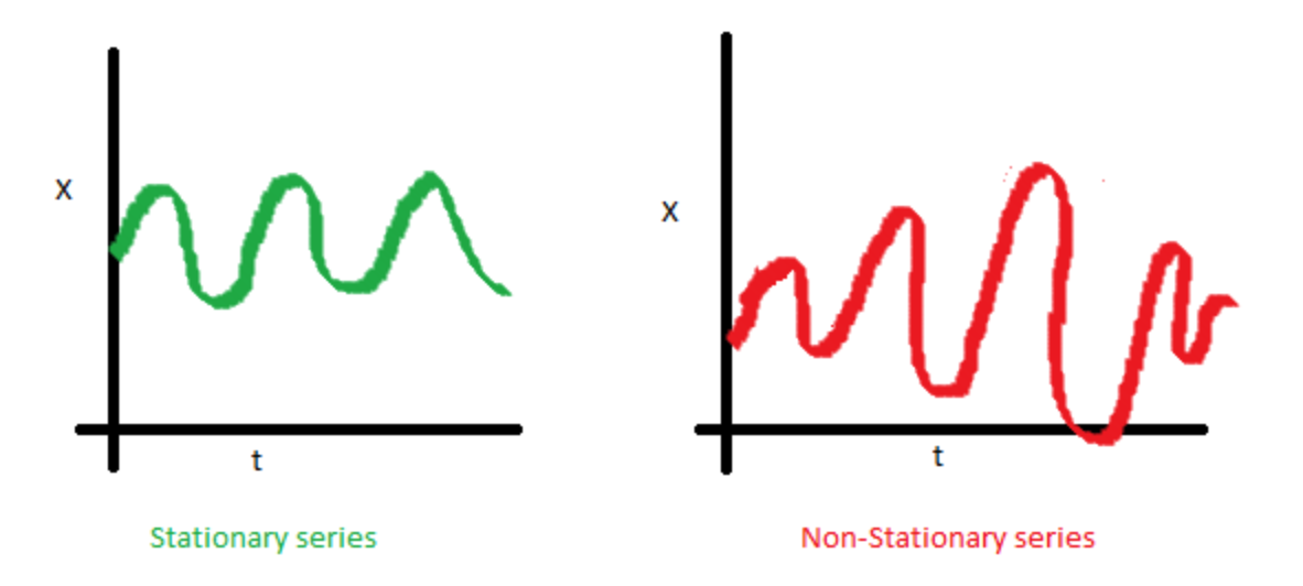
- The covariance of the series data should be constant and can not be explained by time
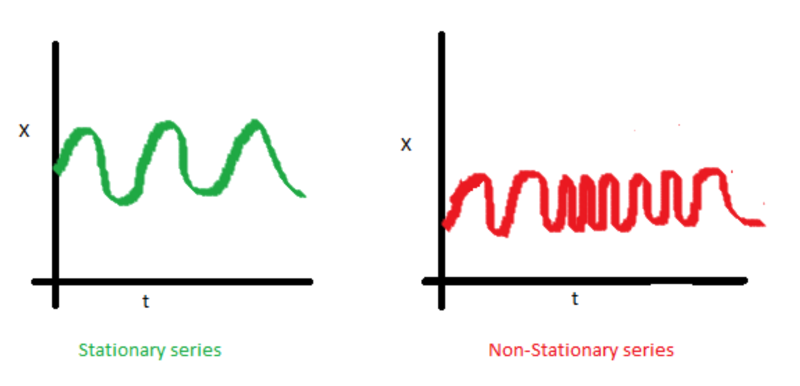
- The mean of the series data should be constant and can not be explained by time
Single Exponential Smoothing
- Data Assumptions:
\[\{y_t,\; t=1,2,...\}\] is a stationary time series which has properties that \(P(Y_{t_1})=P(Y_{t_2}),\; \forall t_1,\,t_2=1,2,...\) and then \(E(Y_{t_1})=E(Y_{t_2}),\; \forall t_1,\,t_2=1,2,...\).
if(!require("forecast")) install.packages("forecast")
library(forecast)
mean = 100
set.seed(123)
res = rnorm(n = 240, mean = 0, sd = 5)
myvector = mean + res
dat = ts(myvector, start=c(2017, 1), frequency=12)
fit = HoltWinters(dat, beta=FALSE, gamma=FALSE)
fit_h = forecast(fit, h=10)
par(mfrow = c(1, 2))
plot(stl(dat, s.window=12), main="Single Exponential Smoothing")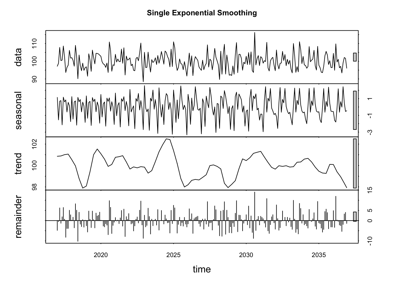
par(mfrow=c(2,2))
plot(fit)
plot(fit_h)
acf(fit_h$residuals, na.action = na.omit)
pacf(fit_h$residuals, na.action = na.omit)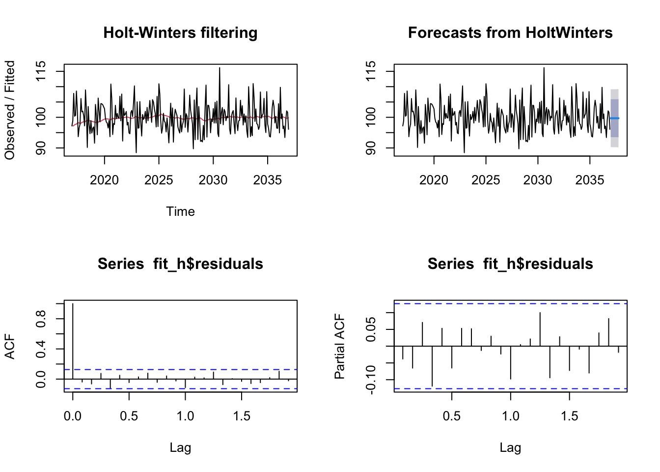
Algorithm:
The original algorithm which was defined by Winters (1960),\[ \begin{align} \hat{y_{t}} &= \alpha y_t + (1-\alpha)\hat{y_{t-1}} \:, \quad 0< \alpha \leq 1 \\ \end{align} \]
The alternative algorithm which has the same property as the original one but makes more sense on explanation,
\[ \begin{align} \hat{y_{t}} &= \alpha y_{t-1}+ (1-\alpha)\hat{y_{t-1}} \:, \quad 0< \alpha \leq 1 \\[5pt] \hat{y_{t+h}} &= \hat{y_{t+1}} \\[5pt] &= \alpha y_{t}+ (1-\alpha)\hat{y_{t}} \end{align} \]
Initial values:
To initiate the single exponential smoothing, we should give a initial value, \(\hat{y_0}\). There are many methods to choose the initial value, like \(\hat{y_0}=y_0\) or the mean value of the first \(n\) time points, \(\hat{y_0}=\frac{1}{n}\sum_{i=1}^{n}y_i\).Parameters:
\[{\alpha}\]
The common method for calculating \(\alpha\) is finding the estimates which can minimizing Sum of the Square of Errors (SSE), \(\sum_{i=1}^{n}(y_i-\hat{y_i})^2\), or Mean Square of Errors (MSE), \(\frac{1}{n}\sum_{i=1}^{n}(y_i-\hat{y_i})^2\).Derivation:
The derivation of the original algorithm can be found in Winters (1960). The following is the proof for the alternative one based on Winters’s derivation ideas. Here, we can suppose \(y_t\) are random variables.
\[ \begin{align} \hat{y_1} &= \alpha y_0 + (1-\alpha) \hat{y_0} \\[5pt] \hat{y_2} &= \alpha y_1 + (1-\alpha) \hat{y_1} \\[5pt] &= \alpha y_1 + (1-\alpha)(\alpha y_0 + (1-\alpha) \hat{y_0}) \\[5pt] &= \alpha y_1 + \alpha(1-\alpha)y_0 + (1-\alpha)^2 \hat{y_0} \\[5pt] &\quad \quad \quad \vdots \\[5pt] \hat{y_t} &= \alpha y_{t-1} + \alpha (1-\alpha)y_{t-2} + \alpha (1-\alpha)^2 y_{t-3} +\dots + \\[5pt] &\qquad \alpha (1-\alpha)^{t-2}y_1 + \alpha(1-\alpha)^{t-1}y_0 + (1-\alpha)^t\hat{y_0} \\[5pt] &= \alpha\sum_{i=1}^{t} (1-\alpha)^{i-1}y_{t-i} + (1-\alpha)^t\hat{y_0} \\[10pt] \text{Then} \quad E(\hat{y_t}) &= \alpha\sum_{i=1}^{t} (1-\alpha)^{i-1}E(y_{t-i}) + (1-\alpha)^tE(\hat{y_0}) \\[5pt] \text{(when $t$ is large, $(1-\alpha)^t$ }&\text{will approach to $0$ and $\alpha\sum_{i=1}^{t} (1-\alpha)^{i-1}$ will approach to $1$.)} \\[5pt] &\simeq E(y_{t-i}) = E(y_t) \text{ (which meets the assumption of stationary process.)} \end{align} \]
- Data Assumptions:
Double Exponential Smoothing
- Data Assumptions:
Unlike the data assumption of Single Exponential Smoothing, Double Exponential Smoothing allows data has trend feature. That is, data points has stationary process on a line with trend.
mean = 100
set.seed(123)
res = rnorm(n = 240, mean = 0, sd = 5)
trend = 0.2*c(1:240)+5
myvector = mean + res + trend
dat = ts(myvector, start = c(2017, 1), frequency = 12)
fit = HoltWinters(dat, gamma = FALSE)
fit_h = forecast(fit, h=10)
par(mfrow = c(1, 2))
plot(stl(dat, s.window=12), main="Double Exponential Smoothing")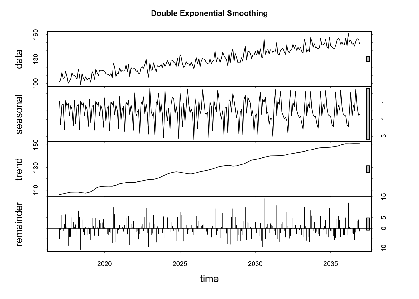
par(mfrow = c(2,2))
plot(fit)
plot(fit_h)
acf(fit_h$residuals, na.action = na.omit)
pacf(fit_h$residuals, na.action = na.omit)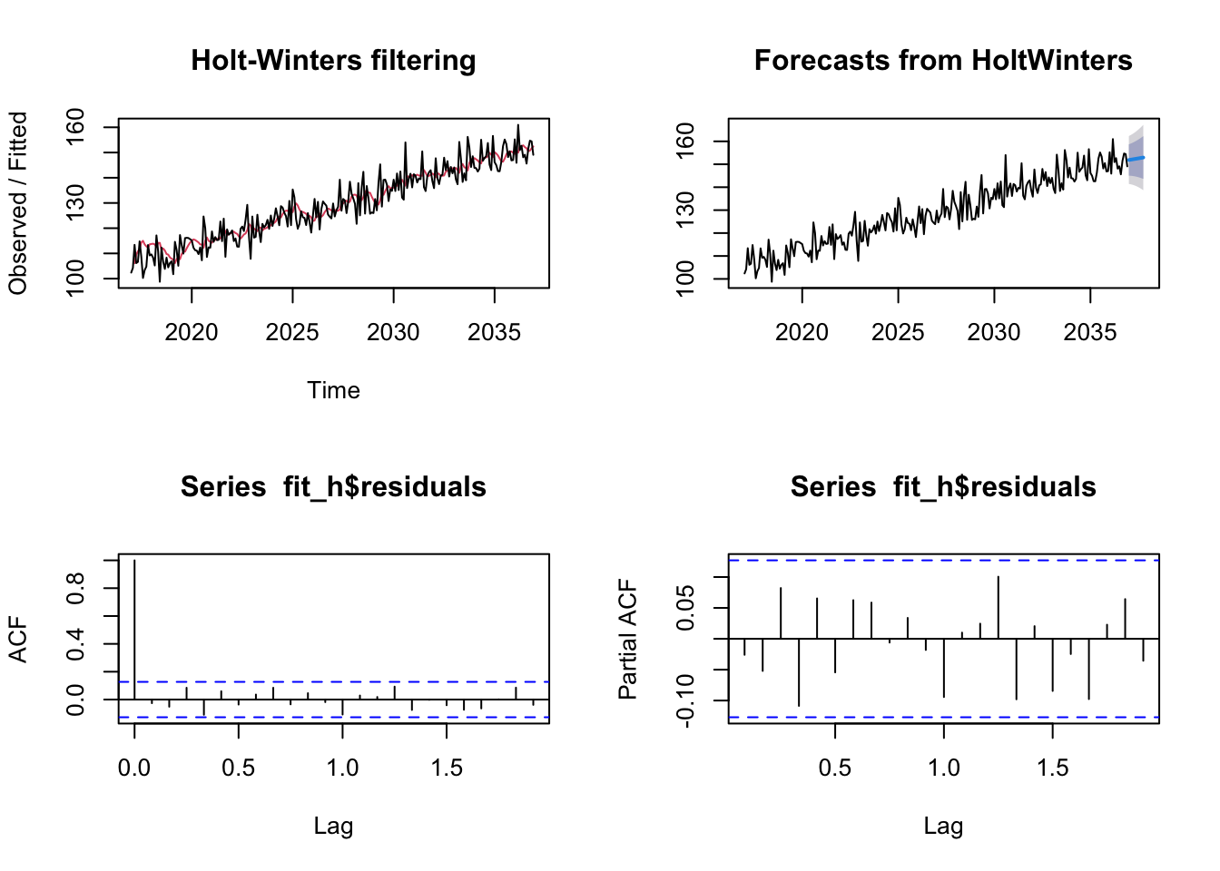
Algorithm:
\[ \begin{align} \text{level:}& &&l_{t} = \alpha y_{t} + (1-\alpha) (l_{t-1}+b_{t-1}) \\[5pt] \text{trend:}& &&b_{t} = \beta (l_t-l_{t-1}) + (1-\beta) b_{t-1} \\[5pt] \text{prediction:}& &&\hat{y_{t+1}} = l_{t}+b_{t} \\[5pt] & &&\hat{y_{t+h}} = l_t + hb_t \end{align} \]
Initial Values:
The inital values are \(l_0\) and \(b_0\).Parameters:
\[{\alpha, \beta}\]
The common method for calculating \(\alpha\) is finding the estimates which can minimizing Sum of the Square of Errors (SSE), \(\sum_{i=1}^{n}(y_i-\hat{y_i})^2\), or Mean Square of Errors (MSE), \(\frac{1}{n}\sum_{i=1}^{n}(y_i-\hat{y_i})^2\).
- Data Assumptions:
Triple Exponential Smoothing (Holt-Winters Method)
- Data Assumptions:
The data has stationary process on a line with not only trend but also seasonality.
mean = 100
set.seed(123)
res = rnorm(n = 240, mean = 0, sd = 5)
trend = 0.2 * c(1:240) + 5
season = 4 * rep(c(0,1,2,3,2,1,0,-1,-2,-3,-2,-1),240/12)
myvector = mean + res + trend + season
dat = ts(myvector, start=c(2017, 1), frequency=12)
fit = HoltWinters(dat)
fit_h = forecast(fit, h = 12)
par(mfrow = c(1, 2))
plot(stl(dat, s.window = 12), main="Triple Exponential Smoothing")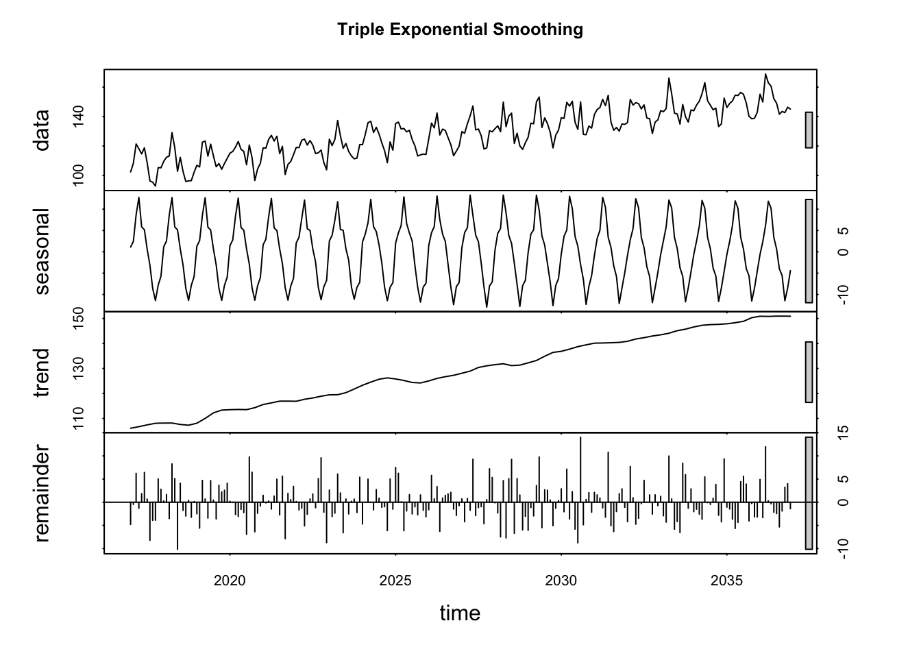
par(mfrow = c(2,2))
plot(fit)
plot(fit_h)
acf(fit_h$residuals, na.action = na.omit)
pacf(fit_h$residuals, na.action = na.omit)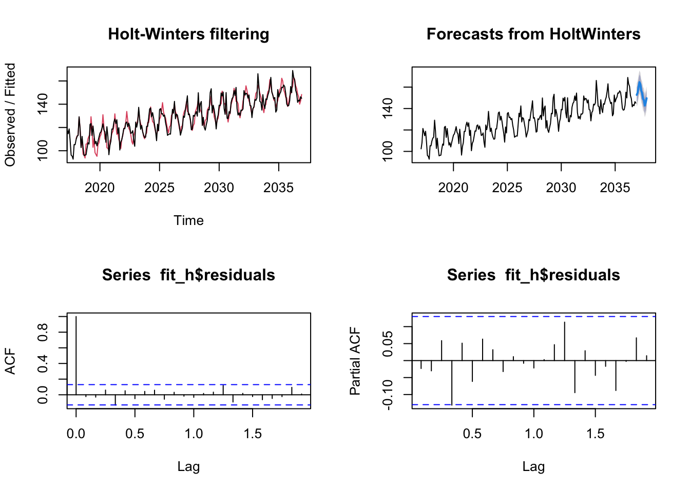
- Algorithm:
\[ \begin{align} \quad \text{level:}& &&l_{t} = \alpha (y_{t}-s_{t-m}) + (1-\alpha) (l_{t-1}+b_{t-1}) \\[5pt] \quad \text{trend:}& &&b_{t} = \beta (l_t-l_{t-1}) + (1-\beta) b_{t-1} \\[5pt] \text{seasonal:}& &&s_{t} = \gamma(y_{t}-l_{t-1}-b_{t-1})+(1-\gamma)s_{t-m} \\[5pt] & &&\text{where $m$ is the length of seasonality} \\[5pt] \text{prediction:}& &&\hat{y_{t+1}} = l_{t}+b_{t}+s_{t-m} \\[5pt] & && \hat{y_{t+h}} = l_t + hb_t +s_{t-m+h_m^+}\;, \\[5pt] & &&\text{where $h_m^+ = [(h−1) \text{ mod } m]+1$} \end{align} \]
Initial Values:
The inital values are \(l_0\), \(b_0\), \[\{s_0^1, s_0^2, ...s_0^m\}\].Parameters:
\[{\alpha, \beta, \gamma}\]
The common method for calculating \(\alpha\) is finding the estimates which can minimizing Sum of the Square of Errors (SSE), \(\sum_{i=1}^{n}(y_i-\hat{y_i})^2\), or Mean Square of Errors (MSE), \(\frac{1}{n}\sum_{i=1}^{n}(y_i-\hat{y_i})^2\).
- Data Assumptions:
Other Forms of Exponential Smoothing Methods
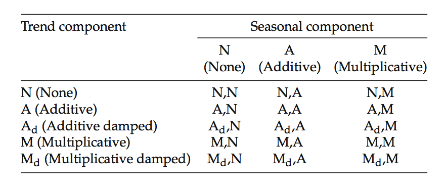
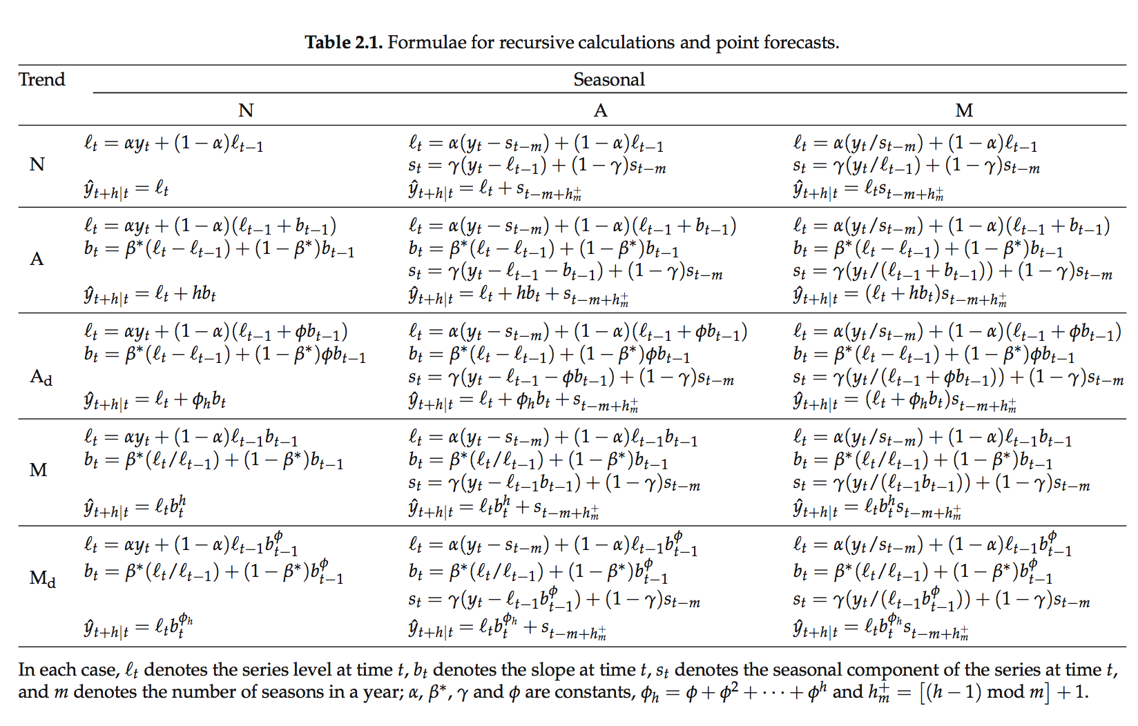
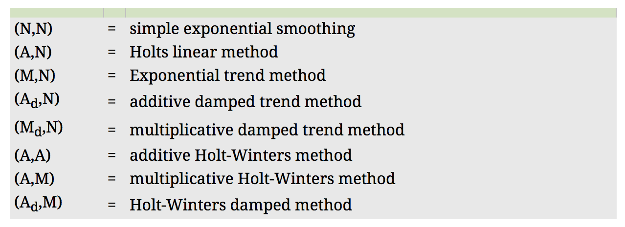
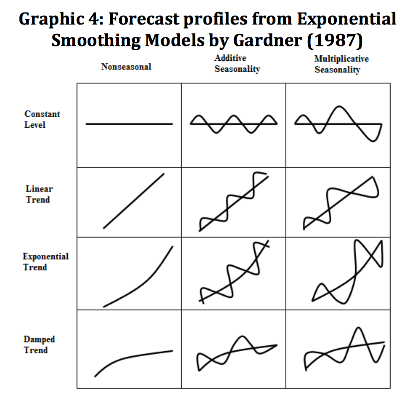
The above Double and Triple Exponential Smoothing are the simplest case. Prof. Hyndman has listed out all the current 15 forms of Exponential Smoothing models in his book, Forecasting with Exponential Smoothing: The State Space Approach (2008). The tables are from the p.12 and p.18 of this book. In his book, he also has wonderful explanations for every model. The last table is from his another book, Forecasting: Principles and practice (2013). The graph is “forecast profile” which I got from Dimitrov (2013) but originated from Garden(1987).
Strengths and Weaknesses
- Strengths
- The alogrithm is explicit and easy to be understood.
- Can be computed quick.
- More weight on recent data.
- Good at short-term forecasts.
- Weaknesses
- Need to do research on finding initial values.
- Not good at mid-term and long-term forecasts.
- Can not add explanotary variables.
- Can not construct prediction interval but only point prediction.
- It is hard to meet the data assumptions of stationary but it is still a referable method of prediction.
- Strengths
Further Topics
- Multi-seasonality:
Taylor (2003, 2008) extended Triple Exponential Smoothing model to double and multiple seasonality.
- Multi-seasonality: