State Space Model for Exponential Smoothing

Time Series Analysis

The main weakness of original Exponential Smoothing Method is that it can only provide point estimation. Hyndman (2002) proposed using state space framework to rewrite the original exponential smoothing algorithm and then give distribution assumption on the error terms to calculate the prediction interval. There are two types of error terms in the state space model: Additive and Multiplicative. The point estimator for these two models are the same but the prediction intervals are different.

This post is my note about learning State Space Model for Exponential Smoothing. All the contents in this post are based on my reading on many resources which are listed in the References part.

References

Paper
- Hyndman, Rob J., Anne B. Koehler, Ralph D. Snyder, and Simone Grose. “A state space framework for automatic forecasting using exponential smoothing methods.” International Journal of Forecasting 18, no. 3 (2002): 439-454.
Book
- Forecasting with Exponential Smoothing: The State Space Approach (2008)

Details

15 Forms of Exponential Smoothing Methods
This table are from the p.18 of the book, Forecasting with Exponential Smoothing: The State Space Approach (2008).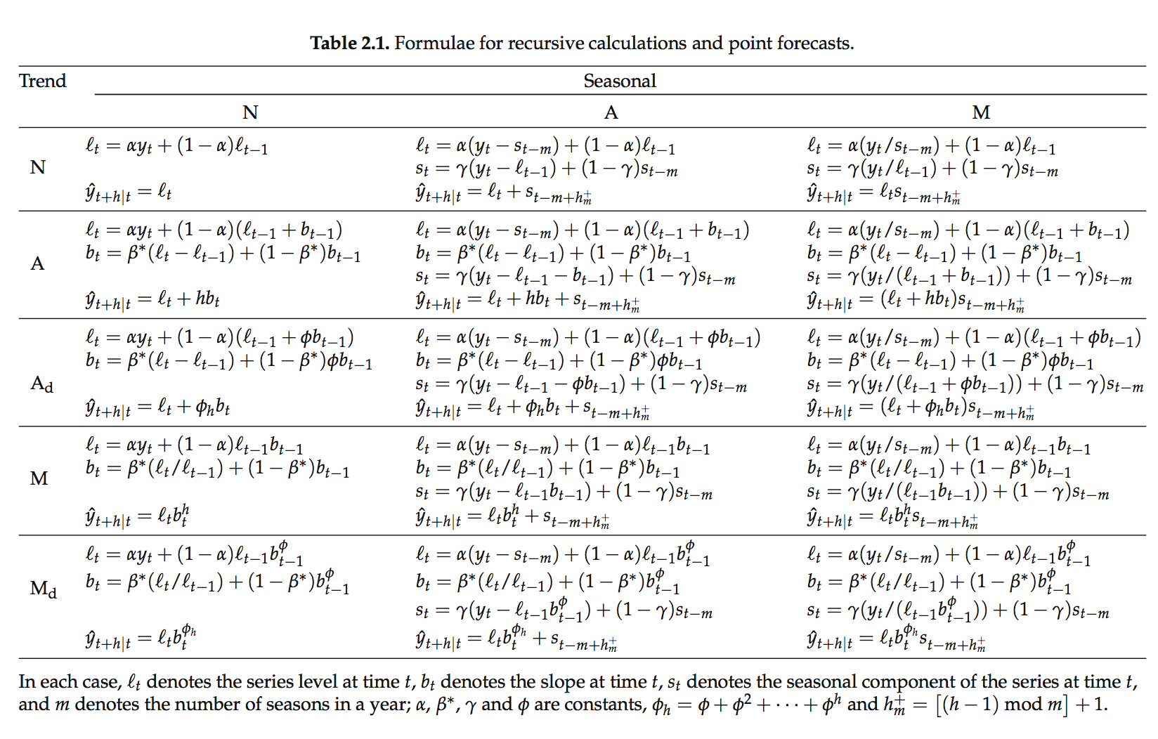
State Space Model
There are two types of State Space model: Additive and Multiplicative Error terms. And the original 15 Forms of Exponential Smoothing Methods can be reexpress in the form of either State Space Model form.
- Algorithm
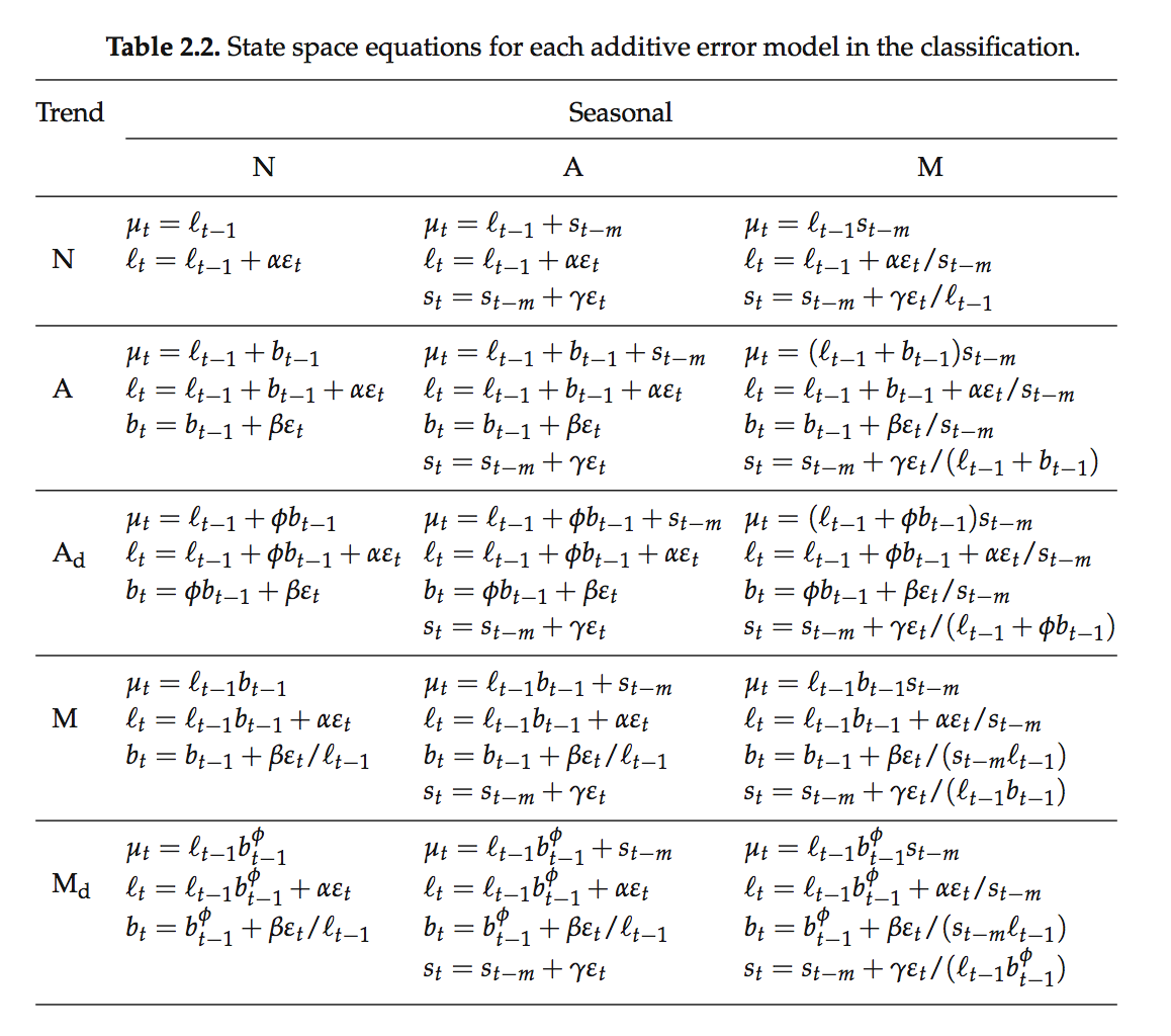
  1. Additive Error
    We assume,
    
    \[ \begin{align} \varepsilon_t &= y_t-\mu_t = y_t - \hat{y_t} \\[5pt] \varepsilon_t &\sim NID(0,\sigma^2) \end{align} \]
    
    and then plug \[y_t = \hat{y_t} + \varepsilon _t\] into the original 15 Forms of Exponential Smoothing Methods, we can get their model expression in the additive state space form. The table are from the p.21 of the book, Forecasting with Exponential Smoothing: The State Space Approach (2008).
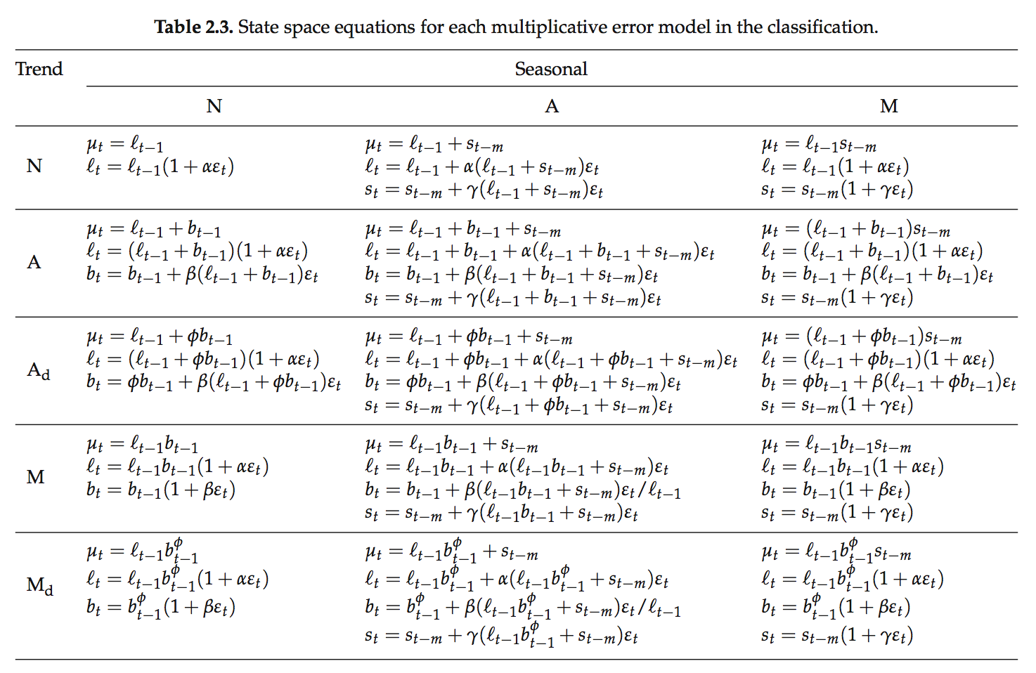
  2. Multiplicative Error
    We assume,
    
    \[ \begin{align} \varepsilon_t &= \frac{y_t-\mu_t}{\mu_t} =\frac{y_t-\hat{y_t}}{\hat{y_t}} \\[5pt] \varepsilon_t &\sim NID(0,\sigma^2) \end{align} \]
    
    and then plug \[y_t = \hat{y_t} + \hat{y_t}\varepsilon _t = \hat{y_t}(1+\varepsilon _t)\] into the original 15 Forms of Exponential Smoothing Methods, we can get their model expression in the multiplicative state space form. The table are from the p.22 of the book, Forecasting with Exponential Smoothing: The State Space Approach (2008).
- Initial Values:
  The inital values are \(l_0\), \(b_0\), \(\{s_0^1, s_0^2, ...s_0^m\}.\) Hyndman (2002) proposed a complete scheme to find out the initial values.
- Parameters:
  \(\alpha\), \(\beta\), \(\gamma\), \(\phi\).
  Under the Guassian assumption of \(\varepsilon _t\), the parameters can be estimated by maximizing the loglikelihood function or minimizing the one-step Mean Square of Errors (MSE), \(\frac{1}{n}\sum_{i=1}^{n}(y_i-\hat{y_i})^2\) and so on. The model selection method is using \(AIC = 2p + 2ln(L).\) More information about AIC : Facts and fallacies of the AIC, Wikipedia
- Strengths and Weaknesses
  - Strengths
    1. Can not only get point prediction but also interval prediction.
    2. No need to worry about initial values. Can use the scheme proposed by Hyndman (2002).
    3. The point estimator of Additive and Multiplicative models are identical but their prediction intervals are different.
  - Weaknesses
    1. The assumption of \(\varepsilon_t \sim NID(0,\sigma^2)\) may not hold.
    2. Residuals may have autocorrelation.
    3. Can not add explanotary variables.
    4. The periods of multiseaonality should be nested.
    5. For high frequency seasonality, the parameter will be very large.
Further Topics
- Multi-seasonality:
  In the Chapter 14 of Forecasting with Exponential Smoothing: The State Space Approach (2008), Hyndman has talked about how to add multi-seasonality in the State Space Model.