BATS model is Exponential Smoothing Method + Box-Cox Transformation + ARMA model for residuals. The Box-Cox Transformation here is for dealing with non-linear data and ARMA model for residuals can de-correlated the time series data. Alysha M.(2010) has proved that BATS model can improve the prediction performance compared to the simple Sate Space Model. However, BATS model does not do well when the the seaonality is complex and high frequency. So, Alysha M.(2011) propsed TBATS model which is BATS model + Trigonometric Seasonal. The trigonometric expression of seasonality terms can not only dramatically reduced the parameters of model when the frequencies of seaonalities are high but also give the model more flexibility to deal with complex seasonality. In a nutshell, this is how the story goes: Exponential Smoothing Method \(\Rightarrow\) State Space Model \(\Rightarrow\) BATS \(\Rightarrow\) TBATS.
This post is my note about learning BATS and TBATS models. All the contents in this post are based on my reading on many resources which are listed in the References part.
References
- Paper
- De Livera, Alysha M. “Automatic forecasting with a modified exponential smoothing state space framework.” Monash Econometrics and Business Statistics Working Papers 10, no. 10 (2010).
- De Livera, Alysha M., Rob J. Hyndman, and Ralph D. Snyder. “Forecasting time series with complex seasonal patterns using exponential smoothing.” Journal of the American Statistical Association 106, no. 496 (2011): 1513-1527.
- Books
Details
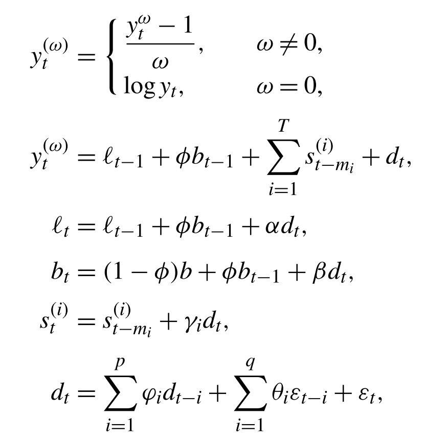
- BATS (Box-Cox Transformation, ARMA residuals, Trend and Seasonality)
Algorithm
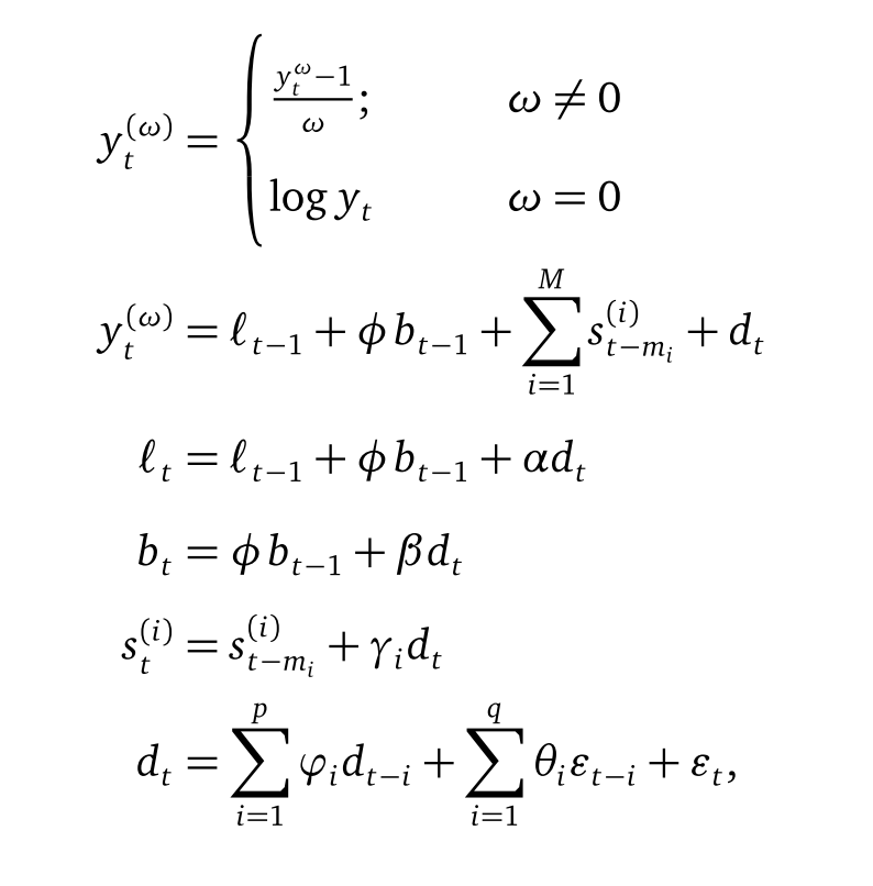
\(\varepsilon_t \sim NID(0,\sigma^2),\) where \(i = \text{the } ith \text{ seasonality}.\) If it is double seasonality then \(i = 1, 2.\)
Initial Values:
The inital values are \(l_0\), \(b_0\), \(\{s_0^1, s_0^2, ...s_0^{m_1}\}\), \(\{s_0^1, s_0^2, ...s_0^{m_2}\}\), …\(\{s_0^1, s_0^2, ...s_0^{m_k}\}\). The \(k\) here is the total number of seasonality. Alysha M.(2010) has a thorough explanation about finding initial values for different cases in her paper.Parameters:
\(\omega,\;\phi,\;\alpha,\;\beta,\;\gamma_1,\cdots,\gamma_k,\;\varphi_1,\cdots,\varphi_p\;,\theta_1,\cdots,\theta_q.\)
Under the Guassian assumption of \(\varepsilon _t\), the parameters can be estimated by maximizing the loglikelihood function or minimizing the Mean Square of Errors (MSE), \(\frac{1}{n}\sum_{i=1}^{n}(y_i-\hat{y_i})^2\) and so on. The \(p,\;q\) here can be \(0,\;1,\;2,3\;,4,\;5\). Choose the one by minimizing the \(AIC = 2p + 2ln(L)\). More information about AIC : Facts and fallacies of the AIC, WikipediaStrengths and Weaknesses
- Strengths
- Box-cox transformation can deal with data with non-linearity and then somewhat makes the variance becomes constant.
- ARMA model on residuals can solve autocorrelation problem.
- No need to worry about initial values.
- Can get not only point prediction but also interval prediction.
- The performance is better than simple state space model.
- Weaknesses
- The assumption of \(\varepsilon_t \sim NID(0,\sigma^2)\) may not hold.
- Can not add explanotary variables.
- The periods of multiseaonality should be nested.
- For high frequency seasonality, the parameter will be very large.
- Strengths
- TBATS (Trigonometric Seasonal, Box-Cox Transformation, ARMA residuals, Trend and Seasonality)
Algorithm:
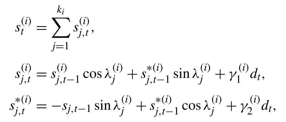 \[\varepsilon_t \sim NID(0,\sigma^2),\] where \(i = \text{the } ith \text{ seasonality}.\) If it is double seasonality then \(i = 1, 2.\)
Initial Values:
Alysha M.(2011) has a thorough explanation about finding initial values after using trigonometric expression to seasonality.Parameters:
\(\omega,\;\phi,\;\alpha,\;\beta,\;\gamma_1,\cdots,\gamma_k,\;\varphi_1,\cdots,\varphi_p\;,\theta_1,\cdots,\theta_q.\)
The method to estimate the parameters are similar to the above BATS modelStrengths and Weaknesses
- Strengths
- Can deal with data with non-integer seasonal period, non-nested periods and high frequency data.
- Can do multi-seasonality without increasing too much parameters.
- All the strengths that BATS has.
- Weaknesses
- The assumption of \(\varepsilon_t \sim NID(0,\sigma^2)\) may not hold.
- Can not add explanotary variables.
- The performance for long-term prediction is not very well.
- The computation cost is big if the data size is large.
- Strengths