Naive Bayes Classifier is a simple and intuitive method for the classification. The algorithm is based on Bayes’ Theorem with two assumptions on predictors: conditionally independent and equal importance. This technique mainly works on categorical response and explanatory variables. But it still can work on numeric explanatory variables as long as it can be transformed to categorical variables.
This post is my note about Naive Bayes Classifier, a classification teachniques. All the contents in this post are based on my reading on many resources which are listed in the References part.
References
Details
- Name : Naive Bayes Classifier
- Data Type :
- Reponse Variable : Categorical
- Explanatory Variable : Categorical and Numeric
(The numeric variables need to be discretized by binning or using probability density function.)
The below picture originated from : here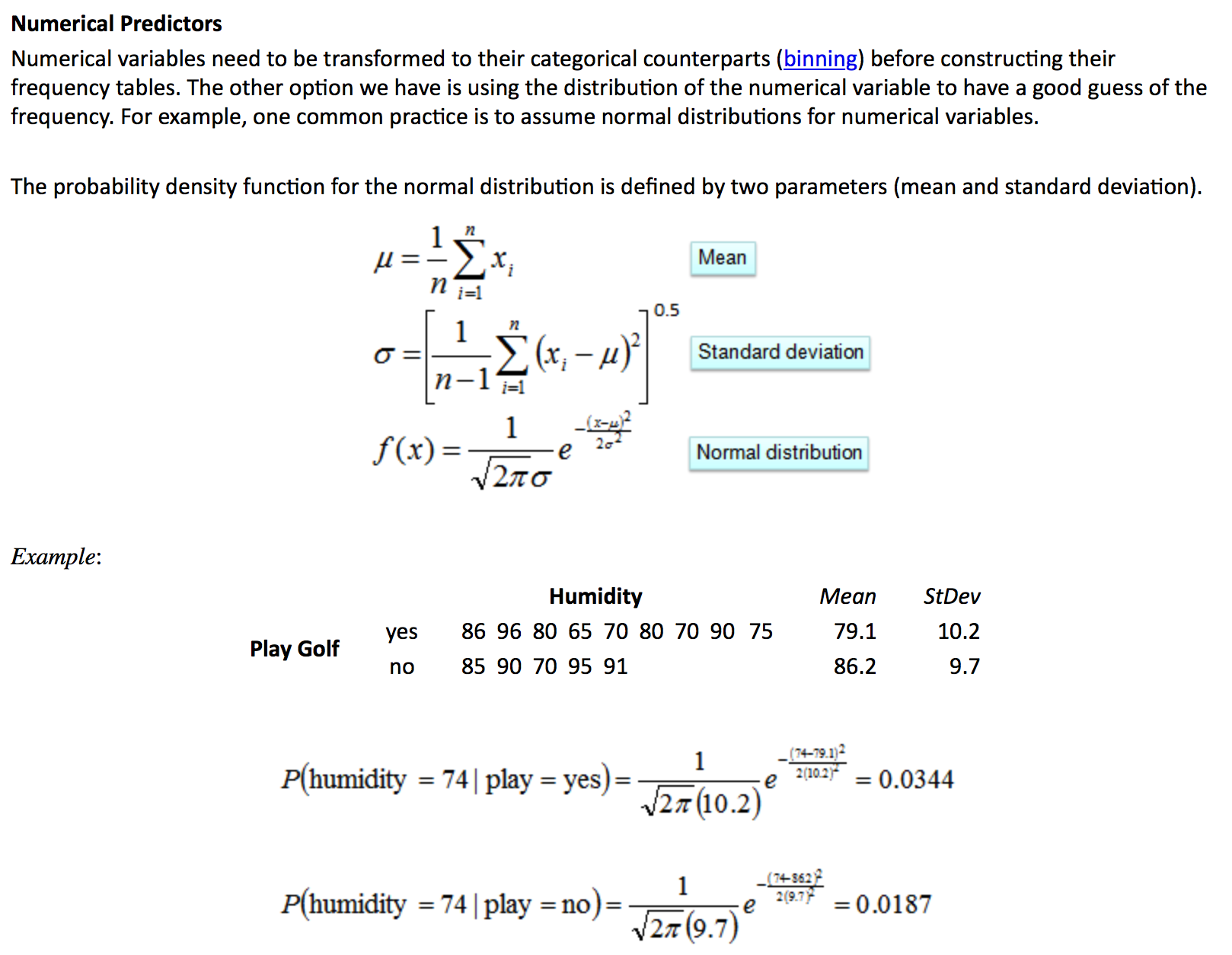
- Reponse Variable : Categorical
- Assumptions :
- All the predictors have equal importance to the response variable.
In other words, all predictors will be put in the algorithm even though some of them may not be as influential as others. - All the predictors are conditionally independent to each other given in any class.
That means, we always treat them conditionally independent no matter it is true or not. For example, suppose we have two datasets. In the first dataset, \(X1\) and \(X2\) given \(Type=A\) is kind of independent to each other, but in the second datset, they are completely dependent to each other.
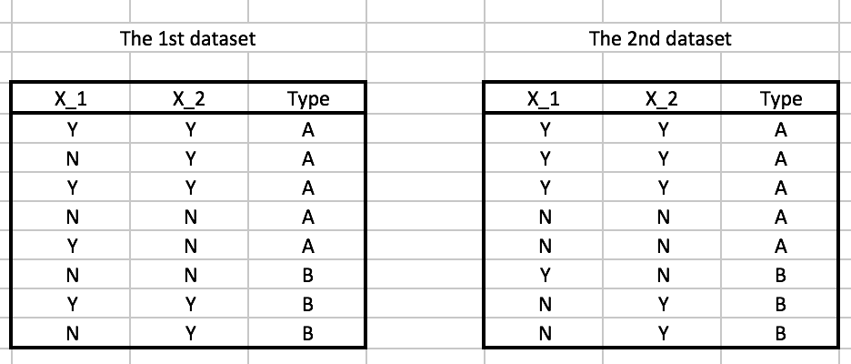
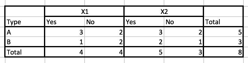
Nevertheless, they all have they same contingency table and will have the same result of Naive Bayes Classifier.
- All the predictors have equal importance to the response variable.
- Bayes’ Theorem
\[ \begin{align} P(A|B) &= \frac{P(A \cap B)}{P(B)} \\[5pt] &= \frac{P(B|A)P(A)}{P(B)} \\[5pt] &= \frac{P(B|A)P(A)}{\sum_{i}^{}P(B|{A}_{i})P({A}_{i})} \end{align} \]
Algorithm
Given a class variable \[Y= \{ 1, 2,..., K \}, K\geq2\] and explanatory variables, \[X=\{ X_1, X_2,..., X_p \}, \] the Bayes’ Theorem can be written as: \[ \begin{align} P(Y=k|X=x) &= \frac{P(X=x|Y=k)P(Y=k)}{P(X=x)} \\[5pt] &= \frac{P(X=x|Y=k)P(Y=k)}{\sum_{i=1}^{K}P(X=x|Y=i)P(Y=i)} \end{align} \]The Naive Bayes Classifier is a function, \[C \colon \mathbb{R}^p \rightarrow \{ 1, 2,..., K \}\] defined as
\[ \begin{align} C(x) &=\underset{k\in \{ 1, 2,..., K \} }{\operatorname{argmax}}P(Y=k|X=x) \\[5pt] &= \underset{k\in \{ 1, 2,..., K \} }{\operatorname{argmax}}P(X=x|Y=k)P(Y=k) \\[5pt] \quad &(\text{by assuming that } X_1,...,X_p \text{ are conditionally independent when given } Y=k, \forall k\in \{ 1, 2,..., K \}) \\[5pt] &= \underset{k\in \{ 1, 2,..., K \} }{\operatorname{argmax}}P(X_1=x_1|Y=k)P(X_2=x_2|Y=k)\cdots P(X_p=x_p|Y=k)P(Y=k) \end{align} \]
Strengths and Weaknesses
- Strengths:
- simple and effective
- Weaknesses:
- hard to meet the assumptions of eaqual important and mutual independence on predictors.
- not good to deal with many numeric predictors.
- Strengths:
A Simple Example
Suppose we have a contingency table like this: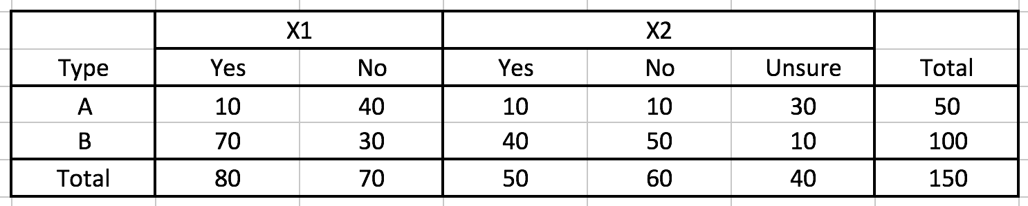
Q : And, what will be our guess on type if we have a data has X1=“Yes” and X2=“Unsure”?
A : Our guess is Type B.
\[ \begin{align} P(A|X_1=\text{"Yes"}, X_2=\text{"Unsure"}) &\propto P(X_1=\text{"Yes"}, X_2=\text{"Unsure"}|A)P(A) \\[5pt] &= P(X_1=\text{"Yes"}|A)P(X_2=\text{"Unsure"}|A)P(A) \\[5pt] &= \frac{10}{50} \cdot \frac{30}{50} \cdot \frac{50}{150} \\[5pt] &= \frac{1}{25} \\[10pt] P(B|X_1=\text{"Yes"}, X_2=\text{"Unsure"}) &\propto P(X_1=\text{"Yes"}, X_2=\text{"Unsure"}|B)P(B) \\[5pt] &= P(X_1=\text{"Yes"}|B)P(X_2=\text{"Unsure"}|B)P(Type=B) \\[5pt] &= \frac{70}{100} \cdot \frac{10}{100} \cdot \frac{100}{150} \\[5pt] &= \frac{14}{300} \\[10pt] C(X_1=\text{"Yes"}, X_2=\text{"Unsure"}) &= \underset{k\in \{ A, B \} }{\operatorname{argmax}}P(Y=k|X_1=\text{"Yes"}, X_2=\text{"Unsure"}) \\[5pt] &= B \end{align} \]
- Further topics
- Laplace Estimator (Machine Learning with R, Chapter 4)
Adding a small number to the frequency table to avoid zero probability for the Naive Bayes Classifier.
- Laplace Estimator (Machine Learning with R, Chapter 4)