LDA and QDA

References

• Books
  1. The Elements of Statistical Learning:Data Mining, Inference, and Prediction
  2. An Introduction to Statistical Learning with Applications in R

Details

• Name
  
  • Linear Discriminant Analysis (LDA)
  • Quadratic Discriminant Analysis (QDA)
    
    
• Data Type
  • Reponse Variable: Categorical
  • Explanatory Variable: Numeric
    
    
• Multivariate Normal Distribution

\[ \begin{align} X \sim N(\mu, \Sigma) &= \frac{1}{(2\pi)^\frac{p}{2}|\Sigma|^\frac{1}{2}}\exp(-\frac{1}{2}(X-\mu)^T\Sigma^{-1}(X-\mu)) \end{align} \]

• Assumptions
  

  • LDA:
    Given a class \(k\), the predictors in this class, \(X_k=(X_{1k},X_{2k},\cdots,X_{pk})\), follows multivariate normal distribution with mean \(\mu_k\) and covariance matrix \(\Sigma\). And, the covariance matrix are all the same for all classes.
    \[ \begin{align} P(X=x|Y=k) &= N(\mu_k, \Sigma) \\[5pt] \text{where } \mu_k &= \begin{pmatrix} \mu_{1k}\\ \mu_{2k}\\ \vdots\\ \mu_{pk} \end{pmatrix} \\[5pt] \Sigma &= \begin{pmatrix} \sigma_1^2& \sigma_{12}& \cdots& \sigma_{1p} \\ \sigma_{12}& \sigma_2^2& \cdots& \sigma_{2p}\\ \vdots& \vdots& \ddots& \vdots\\ \sigma_{1p}& \sigma_{2p} & \cdots & \sigma_p^2 \end{pmatrix}, \, \forall \,k \end{align} \]

  • QDA:
    Given a class \(k\), the predictors in this class, \(X_k=(X_{1k},X_{2k},\cdots,X_{pk})\), follows multivariate normal distribution with mean \(\mu_k\) and covariance matrix \(\Sigma_k\). And, the covariance matrix can NOT be the same for all classes.
    \[ \begin{align} P(X=x|Y=k) &= N(\mu_k, \Sigma_k) \\[5pt] \text{where } \mu_k &= \begin{pmatrix} \mu_{1k}\\ \mu_{2k}\\ \vdots\\ \mu_{pk} \end{pmatrix} \\[5pt] \Sigma_k &= \begin{pmatrix} \sigma_{1_k}^2& \sigma_{12_k}& \cdots& \sigma_{1p_k} \\ \sigma_{12_k}& \sigma_{2_k}^2& \cdots& \sigma_{2p_k}\\ \vdots& \vdots& \ddots& \vdots\\ \sigma_{1p_k}& \sigma_{2p_k} & \cdots & \sigma_{p_k}^2 \end{pmatrix} \end{align} \]
    
    

  if (!require("ggplot2")) install.packages("ggplot2")
  if (!require("MASS")) install.packages("MASS")
  if (!require("grid")) install.packages("grid")
  if (!require("gridExtra")) install.packages("gridExtra")

  ########################################
  #### Generate Bivariate Normal Data ####
  ########################################
  set.seed=12345
  bvm=function(m1,m2,sigma1,sigma2,n1,n2){
      d1 <- mvrnorm(n1, mu = m1, Sigma = sigma1 )
      d2 <- mvrnorm(n2, mu = m2, Sigma = sigma2 )
      d=rbind(d1,d2)
      colnames(d)=c("X1","X2")
      d=data.frame(d)
      d$group=c(rep("1",n1),rep("2",n2))
      list(data = d)
  }

  m_1 <- c(0.5, -0.5)
  m_2 <- c(-2, 0.7)
  sigma_1 <- matrix(c(1,0.5,0.5,1), nrow=2)
  sigma_2 <- matrix(c(0.8,-0.7,-0.7,0.8), nrow=2)

  p1=ggplot(bvm(m_1,m_2,sigma_1,sigma_1,n1=2000,n2=2000)$data,
      aes(x=X1, y=X2)) +
      stat_density2d(geom="density2d", aes(color = group),contour=TRUE)+
      ggtitle("Under LDA assumption")
  p2=ggplot(bvm(m_1,m_2,sigma_1,sigma_2,n1=2000,n2=2000)$data,
      aes(x=X1, y=X2)) +
      stat_density2d(geom="density2d", aes(color = group),contour=TRUE)+
      ggtitle("Under QDA assumption")
  grid.arrange(p1, p2, ncol = 2)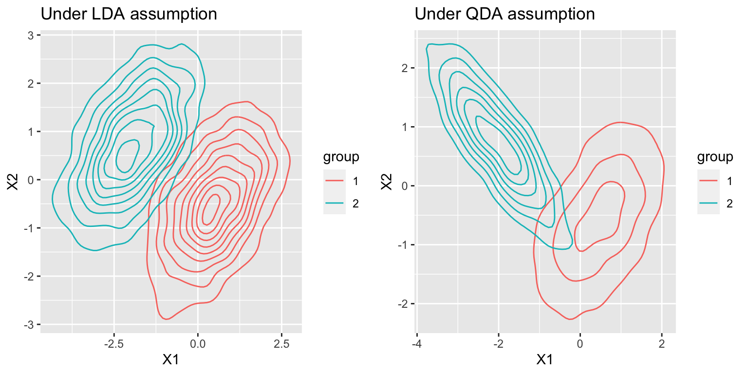

• Algorithm
  Given a class variable \[Y= \{ 1, 2,..., K \}, K\geq2\] and explanatory variables, \[X=\{ X_1, X_2,..., X_p \}, \] the Bayes’ Theorem can be written as:
  

  • LDA:
    

    \[ \begin{align} P(Y=k|X=x) &= \frac{P(X=x|Y=k)P(Y=k)}{P(X=x)} \\[5pt] &= \frac{P(X=x|Y=k)P(Y=k)}{\sum_{i=1}^{K}P(X=x|Y=i)P(Y=i)} \end{align} \]
    
    Then, we define a classifier which is a function, \[C \colon \mathbb{R}^p \rightarrow \{ 1, 2,..., K \}\] and
    
    

    \[ \begin{align} C(x) &=\underset{k\in \{ 1, 2,..., K \} }{\operatorname{argmax}}P(Y=k|X=x) \\[5pt] &= \underset{k\in \{ 1, 2,..., K \} }{\operatorname{argmax}}\log P(Y=k|X=x) \\[5pt] &\propto \underset{k\in \{ 1, 2,..., K \} }{\operatorname{argmax}} \log P(X=x|Y=k) + \log P(Y=k) \\[5pt] \quad &(\text{by assuming that } P(X=x|Y=k) \sim N(\mu_k, \Sigma)) \\[5pt] &= \underset{k\in \{ 1, 2,..., K \} }{\operatorname{argmax}} \log N(\mu_k, \Sigma) + \log P(Y=k) \\[5pt] &= \underset{k\in \{ 1, 2,..., K \} }{\operatorname{argmax}} \log [\frac{1}{(2\pi)^\frac{p}{2}|\Sigma|^\frac{1}{2}}\exp(-\frac{1}{2}(X-\mu_k)^T\Sigma^{-1}(X-\mu_k))] + \log P(Y=k) \\[5pt] &\propto \underset{k\in \{ 1, 2,..., K \} }{\operatorname{argmax}} -\frac{1}{2}(X-\mu_k)^T\Sigma^{-1}(X-\mu_k) + \log (Y=k) \\[5pt] &= \underset{k\in \{ 1, 2,..., K \} }{\operatorname{argmax}} X^T\Sigma^{-1}\mu_k - \frac{1}{2}\mu_k^T\Sigma\mu_k + \log P(Y=k) \\[5pt] &\equiv \underset{k\in \{ 1, 2,..., K \} }{\operatorname{argmax}} \delta_k(x) \end{align} \]
    
    To calculate \(C(X)\), we need to plug in the following estimates which are all unbiased.
    \[ \begin{align} \hat{P}(Y&=k) = \frac{n_k}{n}, \quad \sum_{i=1}^{K}n_i = n \\[5pt] \hat{\mu_k} &= \begin{pmatrix} \hat{\mu_{1k}}\\ \hat{\mu_{2k}}\\ \vdots\\ \hat{\mu_{pk}} \end{pmatrix} = \begin{pmatrix} \bar{X}_{1k} = \frac{1}{n_1}\sum_{i=1}^{n_1}x_{ik}\\ \bar{X}_{2k}\\ \vdots\\ \bar{X}_{pk} \end{pmatrix} \\[5pt] \hat\Sigma &= \text{Pooled Covariance Matrix because of total K classes} \\[5pt] &= \frac{1}{n-K} \sum_{i=1}^{K}\sum_{j=1}^{n_k}(x_{jk}-\hat{\mu_k})(x_{jk}-\hat{\mu_k})^T \end{align} \]
    

  • QDA:
    The function of classifier, \(C(x)\), is as following.
    

    \[ \begin{align} C(x) &=\underset{k\in \{ 1, 2,..., K \} }{\operatorname{argmax}} \log P(Y=k|X=x) \\[5pt] &\propto \underset{k\in \{ 1, 2,..., K \} }{\operatorname{argmax}} \log P(X=x|Y=k) + \log P(Y=k) \\[5pt] \quad &(\text{by assuming that } P(X=x|Y=k) \sim N(\mu_k, \Sigma_k)) \\[5pt] &= \underset{k\in \{ 1, 2,..., K \} }{\operatorname{argmax}} \log N(\mu_k, \Sigma_k) + \log P(Y=k) \\[5pt] &= \underset{k\in \{ 1, 2,..., K \} }{\operatorname{argmax}} \log [\frac{1}{(2\pi)^\frac{p}{2}|\Sigma_k|^\frac{1}{2}}\exp(-\frac{1}{2}(X-\mu_k)^T\Sigma_k^{-1}(X-\mu_k))] + \log P(Y=k) \\[5pt] &\propto \underset{k\in \{ 1, 2,..., K \} }{\operatorname{argmax}} -\frac{1}{2}(X-\mu_k)^T\Sigma_k^{-1}(X-\mu_k) - \frac{1}{2}|\Sigma_k|+\log (Y=k) \\[5pt] &= \underset{k\in \{ 1, 2,..., K \} }{\operatorname{argmax}} -\frac{1}{2}X^T\Sigma_kX+X^T\Sigma_k^{-1}\mu_k - \frac{1}{2}\mu_k^T\Sigma_k\mu_k - \frac{1}{2}|\Sigma_k| + \log P(Y=k) \\[5pt] &\equiv \underset{k\in \{ 1, 2,..., K \} }{\operatorname{argmax}} \delta_k(x) \end{align} \]
    
    The estimators are the same as ones in LDA except for \(\Sigma_k\).
    
    \[ \begin{align} \hat\Sigma_k &= \text{Covariance Matrix in class k} \\[5pt] &= \frac{1}{n_k-1} \sum_{j=1}^{n_k}(x_{jk}-\hat{\mu_k})(x_{jk}-\hat{\mu_k})^T \end{align} \]
    

• Decision Boundary
  

  • LDA:
    The decision boundary of LDA is a straight line which can be derived as below.
    \[ \begin{align} &\delta_k(x) - \delta_l(x) = 0 \\[5pt] &\Rightarrow X^T\Sigma^{-1}(\mu_k-\mu_l) - \frac{1}{2}(\mu_k+\mu_l)^T\Sigma(\mu_k-\mu_l)+\log \frac{P(Y=k)}{P(Y=l)} = 0 \\[5pt] &\Rightarrow b_1x+b_0=0 \end{align} \]

  • QDA:
    The decision boundary of QDA is a quadratic line which can be derived as below.
    \[ \begin{align} &\delta_k(x) - \delta_l(x) = 0 \\[5pt] &\Rightarrow -\frac{1}{2}X^T(\Sigma_k -\Sigma_l)X + X^T(\Sigma_k^{-1}\mu_k-\Sigma_l^{-1}\mu_l)-\frac{1}{2}(\mu_k^T\Sigma_k\mu_k-\mu_l^T\Sigma_l\mu_l)\\[5pt] &\quad -\frac{1}{2}(|\Sigma_k|-|\Sigma_l|)+ \log\frac{P(Y=k)}{P(Y=l)}=0\\[5pt] & \Rightarrow b_2x^2+b_1x+b_0=0 \end{align} \]
    
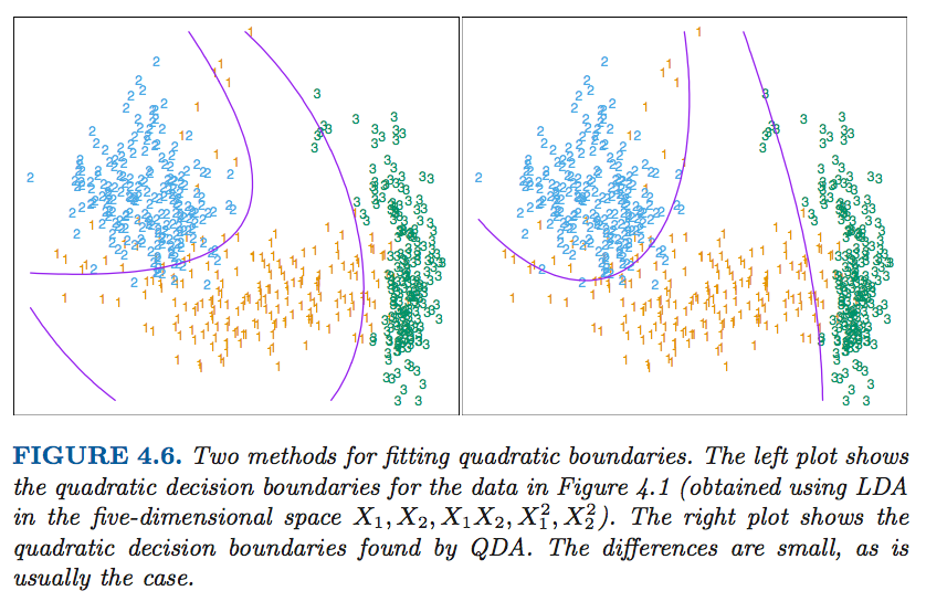
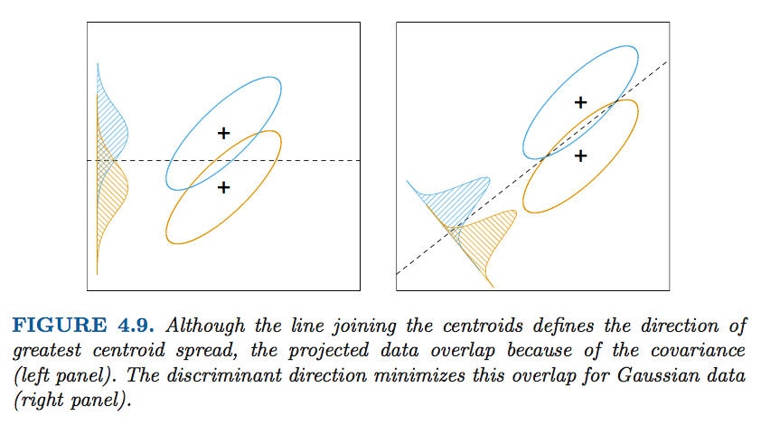
    The following graphs are from The Elements of Statistical Learning:Data Mining, Inference, and Prediction which gave us a clear idea how the decision bounday looks like in LDA and QDA.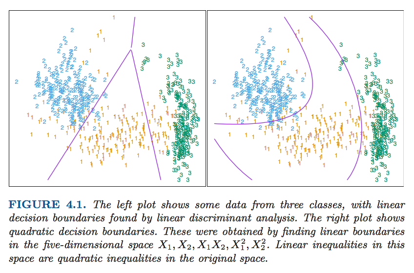

    

• Strengths and Weaknesses
  
  • Strengths:
    
    • It is a simple and intuitive method.
  • Weaknesses:
    
    1. In real life, it is really hard to have a dataset fit the assumption of multivariate normal distribution given classes. But we still can use this method even though the assumption is not met.
    2. It only makes sense when all the predictors are numeric.
• Further topics
  
  • Reduced-Rank Linear Discriminant Analysis (The Elements of Statistical Learning:Data Mining, Inference, and Prediction, p.113 - p.119) This is about finding a decision bounday in LDA to which can maximized between-class variance relatively to the within-class variance.