This post shows the R code for LDA and QDA by using funtion lda() and qda() in package MASS. To show how to use these function, I created a function, bvn(), to generate bivariate normal dataset based on the assumptions and then used lda() and qda() on the generated datasets.
Details
- Resources for Package ‘MASS’
- Example Code
LDA :
Suppose our dataset are from
\[X_{green}=N(\begin{pmatrix} 0.5\\ -0.5 \end{pmatrix}, \Sigma) \quad \text{and} \quad X_{red}=N(\begin{pmatrix} -2\\ 0.7 \end{pmatrix}, \Sigma), \\[5pt] \text{where} \quad \Sigma=\begin{pmatrix} 1& 0.5\\ 0.5&1 \end{pmatrix}.\]QDA :
Suppose our dataset are from
\[X_{green}=N(\begin{pmatrix} -2\\ 0.7 \end{pmatrix}, \Sigma_1) \quad \text{and} \quad X_{red}=N(\begin{pmatrix} 0.5\\ -0.5 \end{pmatrix}, \Sigma_2), \\[5pt] \text{where} \quad \Sigma_1=\begin{pmatrix} 1& 0.5\\ 0.5&1 \end{pmatrix} \quad \text{and} \quad \Sigma_2=\begin{pmatrix} 0.8& -0.7\\ -0.7& 0.8 \end{pmatrix}.\]
if (!require("MASS")) install.packages("MASS")
if (!require("ggplot2")) install.packages("ggplot2")
if (!require("gridExtra")) install.packages("gridExtra")

library(MASS)
library(ggplot2)
library(grid)
library(gridExtra)

########################################
#### Generate Bivariate Normal Data ####
########################################
set.seed(12345)
bvn=function(m1,m2,sigma1,sigma2,n1,n2){
      d1 <- mvrnorm(n1, mu = m1, Sigma = sigma1 )
      d2 <- mvrnorm(n2, mu = m2, Sigma = sigma2 )
      d=rbind(d1,d2)
      colnames(d)=c("X1","X2")
      d=data.frame(d)
      d$group=c(rep("Red",n1),rep("Green",n2))
      list(data = d)
}

m_1 <- c(0.5, -0.5) # mean of the first group
m_2 <- c(-2, 0.7)  # mean of the second group
sigma_1 <- matrix(c(1,0.5,0.5,1), nrow=2) # covariance matrix
sigma_2 <- matrix(c(0.8,-0.7,-0.7,0.8), nrow=2)

# The training dataset
data_lda = bvn(m_1,m_2,sigma_1,sigma_1,n1=1500,n2=2000)$data
data_qda = bvn(m_1,m_2,sigma_1,sigma_2,n1=1500,n2=2000)$data
head(data_lda, 3)
## X1 X2 group
## 1 1.0943941 -0.08022845 Red
## 2 1.4497239 -0.22089273 Red
## 3 0.1516277 -0.34094657 Red###############################
#### Generate Test Dataset ####
###############################
test_lda = bvn(m_1,m_2,sigma_1,sigma_1,n1=100,n2=100)$data
test_qda = bvn(m_1,m_2,sigma_1,sigma_2,n1=100,n2=100)$data
###############################################
#### Scatter Plot of the Generated Dataset ####
###############################################
p1=ggplot(data_lda, aes(x=X1, y=X2)) +
geom_point(aes(colour = group)) +
ggtitle("Dataset for LDA")
p2=ggplot(data_qda, aes(x=X1, y=X2)) +
geom_point(aes(colour = group)) +
ggtitle("Dataset for QDA")
grid.arrange(p1, p2, ncol = 2)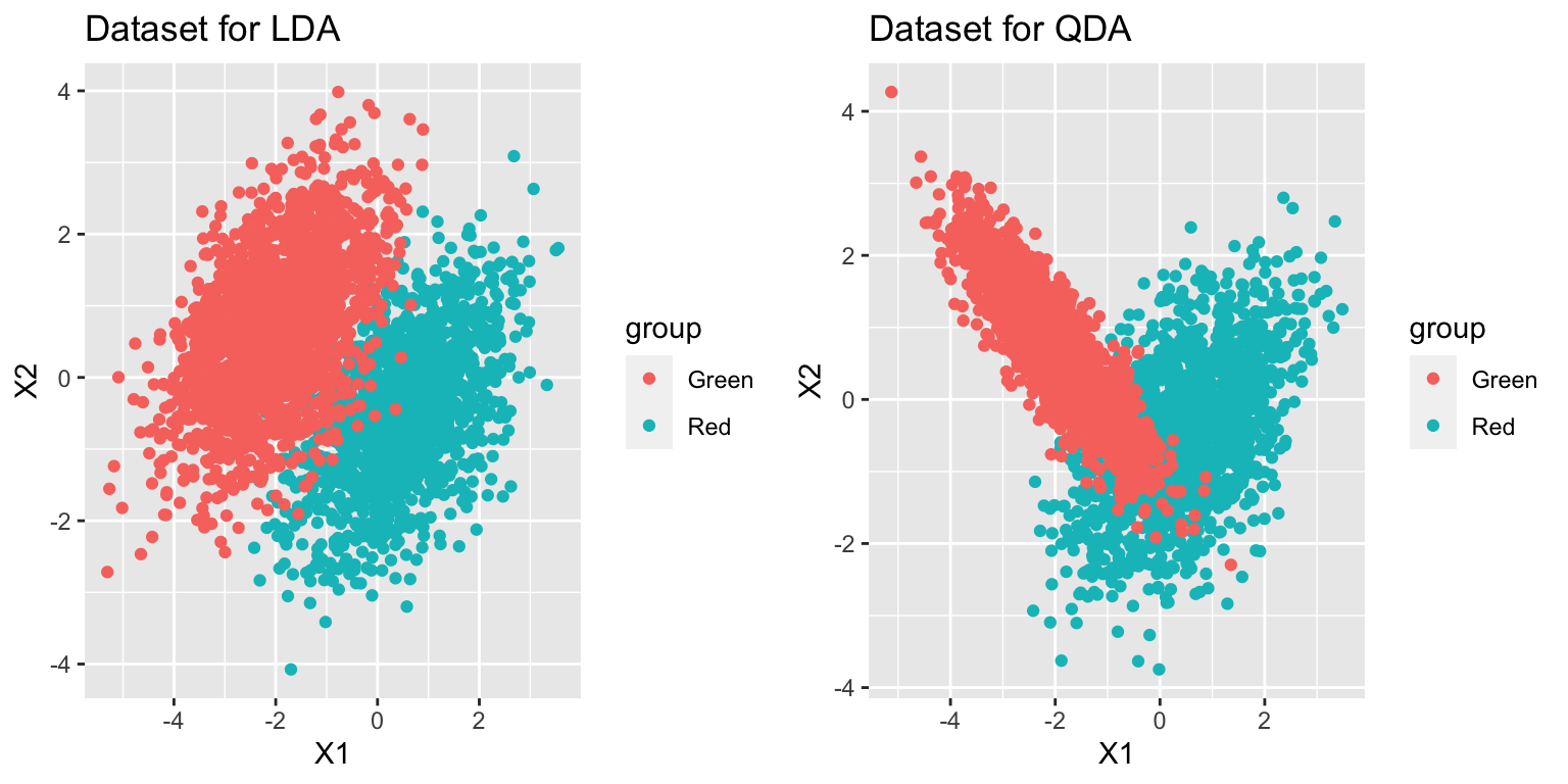
#############
#### LDA ####
#############
m_lda=lda(group~X1+X2, data=data_lda)
m_lda
## Call:
## lda(group ~ X1 + X2, data = data_lda)
##
## Prior probabilities of groups:
## Green Red
## 0.5714286 0.4285714
##
## Group means:
## X1 X2
## Green -1.9873353 0.6966975
## Red 0.5254939 -0.4972749
##
## Coefficients of linear discriminants:
## LD1
## X1 1.1111290
## X2 -0.8491722# The Confusion Matrix
m_lda.pred=predict(m_lda,test_lda)
table(true=test_lda$group, pred=m_lda.pred$class)## pred
## true Green Red
## Green 97 3
## Red 7 93#############
#### QDA ####
#############
m_qda=qda(group~X1+X2, data=data_qda)
m_qda## Call:
## qda(group ~ X1 + X2, data = data_qda)
##
## Prior probabilities of groups:
## Green Red
## 0.5714286 0.4285714
##
## Group means:
## X1 X2
## Green -1.9913743 0.6829456
## Red 0.4691391 -0.4981505# The Confusion Matrix
m_qda.pred=predict(m_qda,test_qda)
table(true=test_qda$group, pred=m_qda.pred$class)## pred
## true Green Red
## Green 98 2
## Red 4 96